Solves a numerical or symbolic system of ordinary differential equations.
ode(
  f,
  var,
  times,
  timevar = NULL,
  params = list(),
  method = "rk4",
  drop = FALSE
)
Arguments
- f
vector of
characters, or afunctionreturning a numeric vector, giving the values of the derivatives in the ODE system at timetimevar. See examples.- var
vector giving the initial conditions. See examples.
- times
discretization sequence, the first value represents the initial time.
- timevar
the time variable used by
f, if any.- params
listof additional parameters passed tof.- method
the solver to use. One of
"rk4"(Runge-Kutta) or"euler"(Euler).- drop
if
TRUE, return only the final solution instead of the whole trajectory.
Value
Vector of final solutions if drop=TRUE, otherwise a matrix with as many
rows as elements in times and as many columns as elements in var.
References
Guidotti E (2022). "calculus: High-Dimensional Numerical and Symbolic Calculus in R." Journal of Statistical Software, 104(5), 1-37. doi:10.18637/jss.v104.i05
See also
Other integrals:
integral()
Examples
## ==================================================
## Example: symbolic system
## System: dx = x dt
## Initial: x0 = 1
## ==================================================
f <- "x"
var <- c(x=1)
times <- seq(0, 2*pi, by=0.001)
x <- ode(f, var, times)
plot(times, x, type = "l")
 ## ==================================================
## Example: time dependent system
## System: dx = cos(t) dt
## Initial: x0 = 0
## ==================================================
f <- "cos(t)"
var <- c(x=0)
times <- seq(0, 2*pi, by=0.001)
x <- ode(f, var, times, timevar = "t")
plot(times, x, type = "l")
## ==================================================
## Example: time dependent system
## System: dx = cos(t) dt
## Initial: x0 = 0
## ==================================================
f <- "cos(t)"
var <- c(x=0)
times <- seq(0, 2*pi, by=0.001)
x <- ode(f, var, times, timevar = "t")
plot(times, x, type = "l")
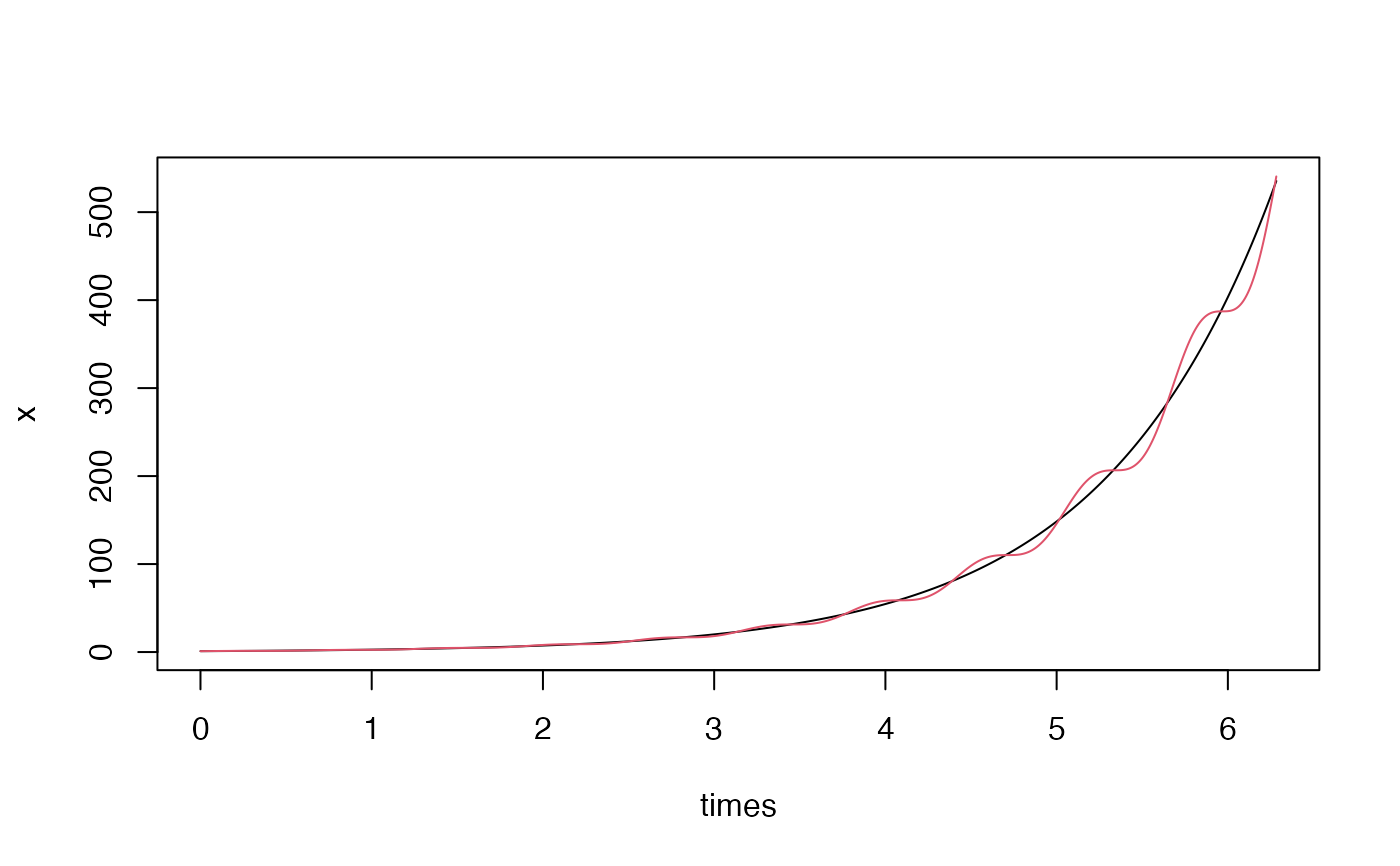
 ## ==================================================
## Example: multivariate time dependent system
## System: dx = x dt
## dy = x*(1+cos(10*t)) dt
## Initial: x0 = 1
## y0 = 1
## ==================================================
f <- c("x", "x*(1+cos(10*t))")
var <- c(x=1, y=1)
times <- seq(0, 2*pi, by=0.001)
x <- ode(f, var, times, timevar = "t")
matplot(times, x, type = "l", lty = 1, col = 1:2)
## ==================================================
## Example: multivariate time dependent system
## System: dx = x dt
## dy = x*(1+cos(10*t)) dt
## Initial: x0 = 1
## y0 = 1
## ==================================================
f <- c("x", "x*(1+cos(10*t))")
var <- c(x=1, y=1)
times <- seq(0, 2*pi, by=0.001)
x <- ode(f, var, times, timevar = "t")
matplot(times, x, type = "l", lty = 1, col = 1:2)
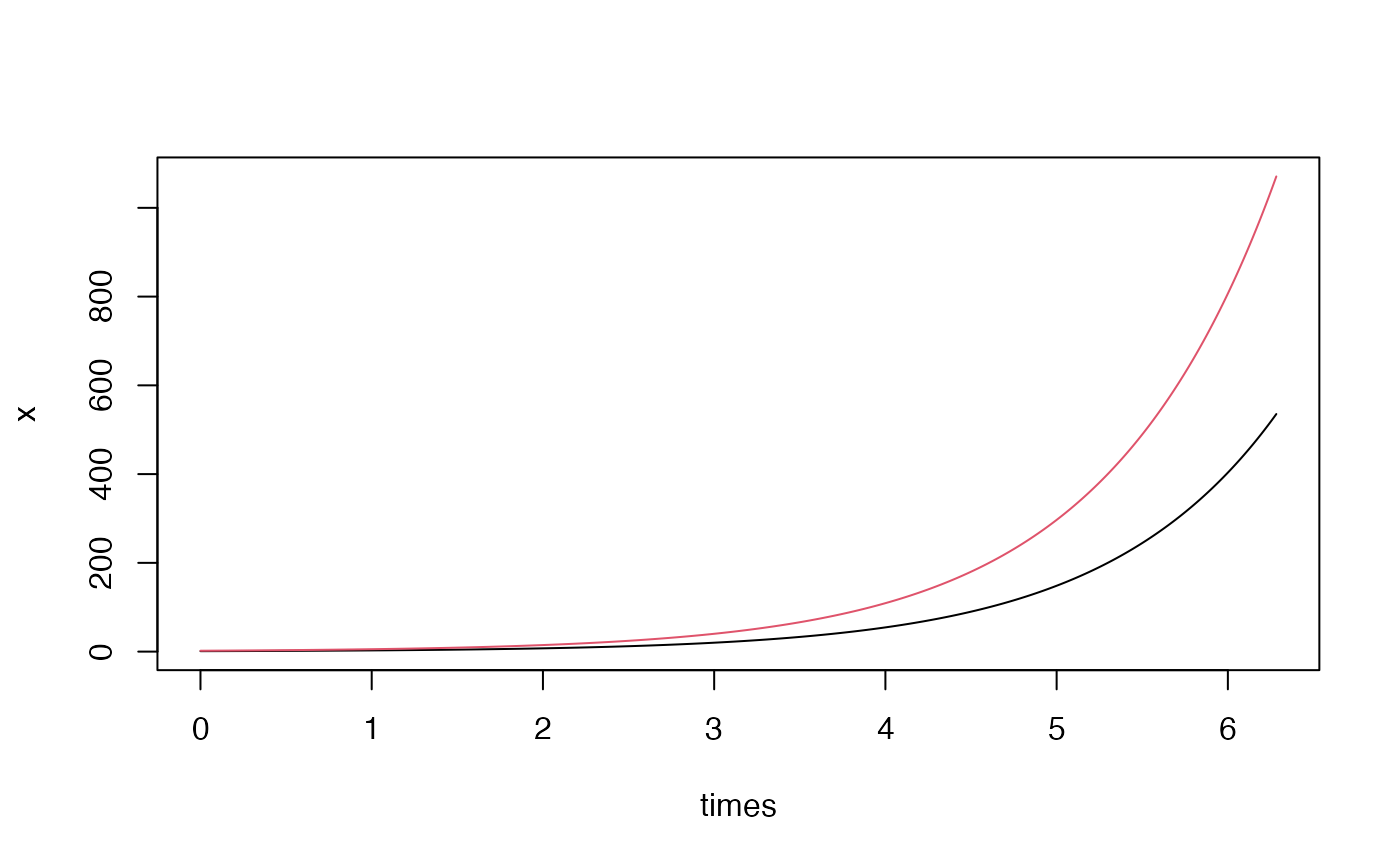
 ## ==================================================
## Example: numerical system
## System: dx = x dt
## dy = y dt
## Initial: x0 = 1
## y0 = 2
## ==================================================
f <- function(x, y) c(x, y)
var <- c(x=1, y=2)
times <- seq(0, 2*pi, by=0.001)
x <- ode(f, var, times)
matplot(times, x, type = "l", lty = 1, col = 1:2)
## ==================================================
## Example: numerical system
## System: dx = x dt
## dy = y dt
## Initial: x0 = 1
## y0 = 2
## ==================================================
f <- function(x, y) c(x, y)
var <- c(x=1, y=2)
times <- seq(0, 2*pi, by=0.001)
x <- ode(f, var, times)
matplot(times, x, type = "l", lty = 1, col = 1:2)
 ## ==================================================
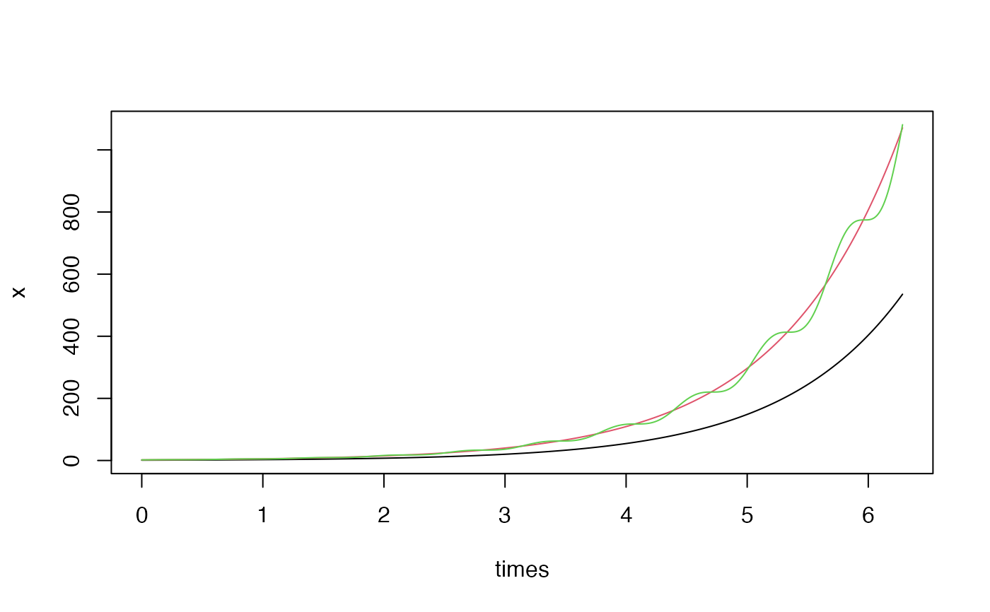
## Example: vectorized interface
## System: dx = x dt
## dy = y dt
## dz = y*(1+cos(10*t)) dt
## Initial: x0 = 1
## y0 = 2
## z0 = 2
## ==================================================
f <- function(x, t) c(x[1], x[2], x[2]*(1+cos(10*t)))
var <- c(1,2,2)
times <- seq(0, 2*pi, by=0.001)
x <- ode(f, var, times, timevar = "t")
matplot(times, x, type = "l", lty = 1, col = 1:3)
## ==================================================
## Example: vectorized interface
## System: dx = x dt
## dy = y dt
## dz = y*(1+cos(10*t)) dt
## Initial: x0 = 1
## y0 = 2
## z0 = 2
## ==================================================
f <- function(x, t) c(x[1], x[2], x[2]*(1+cos(10*t)))
var <- c(1,2,2)
times <- seq(0, 2*pi, by=0.001)
x <- ode(f, var, times, timevar = "t")
matplot(times, x, type = "l", lty = 1, col = 1:3)