The function ode
provides solvers for systems of ordinary differential equations of the
type:
where
is the vector of state variables. Two solvers are available: the simpler
and faster Euler scheme1 or the more accurate 4-th order Runge-Kutta
method2.
Although many packages already exist to solve ordinary differential
equations in R3, they usually represent the function
either with an R function or with characters.
While the representation via R functions is usually more
efficient, the symbolic representation is easier to adopt for beginners
and more flexible for advanced users to handle systems that might have
been generated via symbolic programming. The function ode
supports both the representations and uses hashed
environments to improve symbolic evaluations.
Examples
The vector-valued function
representing the system can be specified as a vector of
characters, or a function returning a numeric
vector, giving the values of the derivatives at time
.
The initial conditions are set with the argument var and
the time variable can be specified with timevar.
Symbolic system
f <- "x"
var <- c(x=1)
times <- seq(0, 2*pi, by=0.001)
x <- ode(f = f, var = var, times = times)
plot(times, x, type = "l")
Time dependent system
f <- "cos(t)"
var <- c(x=0)
times <- seq(0, 2*pi, by=0.001)
x <- ode(f = f, var = var, times = times, timevar = "t")
plot(times, x, type = "l")
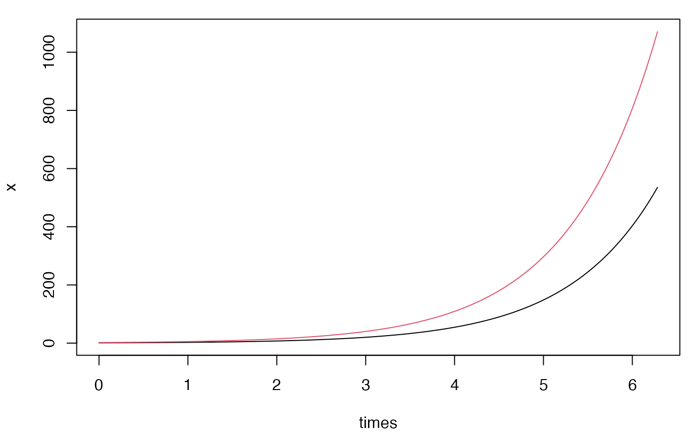
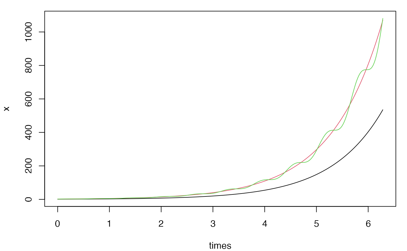
Multivariate system
f <- c("x", "x*(1+cos(10*t))")
var <- c(x=1, y=1)
times <- seq(0, 2*pi, by=0.001)
x <- ode(f = f, var = var, times = times, timevar = "t")
matplot(times, x, type = "l", lty = 1, col = 1:2)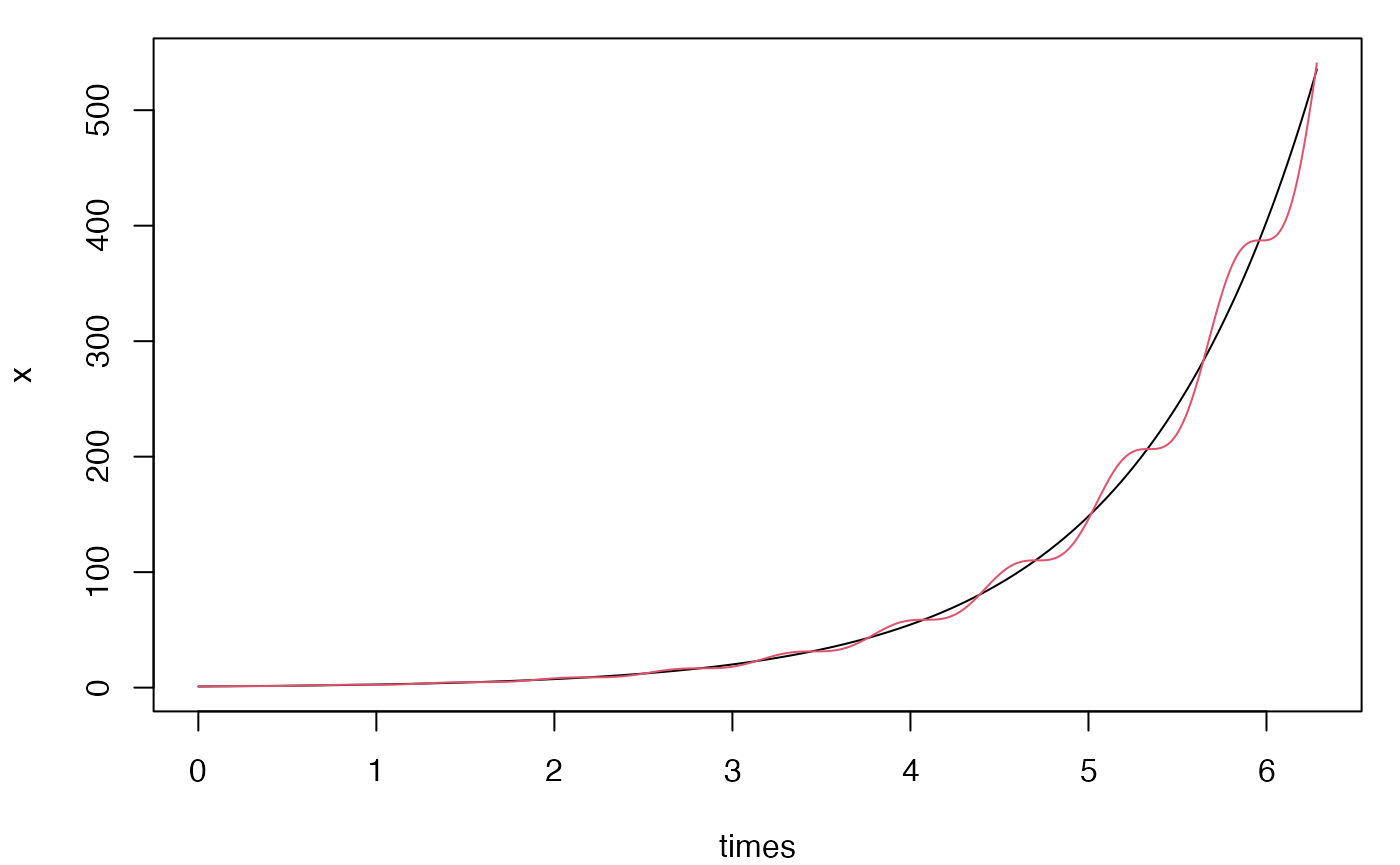
Cite as
Guidotti E (2022). “calculus: High-Dimensional Numerical and Symbolic Calculus in R.” Journal of Statistical Software, 104(5), 1-37. doi:10.18637/jss.v104.i05
A BibTeX entry for LaTeX users is